pacman::p_load(ggstatsplot, ggiraph, plotly, performance, nortest, patchwork, tidyverse)Take-home Exercise 3
Putting Visual Analytics into Practical Use
1. Overview
This exercise aims to unveil the salient patterns in the resale prices of public housing property based on different residential towns and estates through analytical visualization. Appropriate visualization and interactive techniques are applied to enhance users’ data discovery experiences.
In this study, the focus is on 3, 4 and 5 room housing types for the year of 2022.
The dataset used was retrieved from Data.gov.sg, titled Resale flat princes based on registration date from Jan-2017 onwards. The source file is in csv format.
2. Loading R Packages
The following packages and required libraries are loaded in this exercise:
3. Dataset
3.1 Import dataset
#Import dataset from .csv file
HDBdata <- read_csv("Data/resale-flat-prices-based-on-registration-date-from-jan-2017-onwards.csv", show_col_types = FALSE)

#ReView data
head(HDBdata, n=5)
# A tibble: 5 × 11
month town flat_…¹ block stree…² store…³ floor…⁴ flat_…⁵ lease…⁶ remai…⁷
<chr> <chr> <chr> <chr> <chr> <chr> <dbl> <chr> <dbl> <chr>
1 2017-01 ANG MO … 2 ROOM 406 ANG MO… 10 TO … 44 Improv… 1979 61 yea…
2 2017-01 ANG MO … 3 ROOM 108 ANG MO… 01 TO … 67 New Ge… 1978 60 yea…
3 2017-01 ANG MO … 3 ROOM 602 ANG MO… 01 TO … 67 New Ge… 1980 62 yea…
4 2017-01 ANG MO … 3 ROOM 465 ANG MO… 04 TO … 68 New Ge… 1980 62 yea…
5 2017-01 ANG MO … 3 ROOM 601 ANG MO… 01 TO … 67 New Ge… 1980 62 yea…
# … with 1 more variable: resale_price <dbl>, and abbreviated variable names
# ¹flat_type, ²street_name, ³storey_range, ⁴floor_area_sqm, ⁵flat_model,
# ⁶lease_commence_date, ⁷remaining_lease3.2 Data Preparation
From the data review in the earlier step, we want to converting month to date format to do more meaningful analysis. This is done using as.Date() as shown in the code chunk below:
#Appending an artifical day to convert month into date format
HDBdata$month <- paste(HDBdata$month,"01", sep = "-") %>%
  as.Date(HDBdata$month, format = "%Y-%m-%d")
As the dataset contains information that is outside the scope of our studies. We can extract the relevant housing type and time period by using filter() function.
#Filtering the dataset based on time range and flat types
HDBdata2022 <- HDBdata %>% filter(month>"2021-12-01" & month<"2023-01-01") %>%
  filter(flat_type %in% c("3 ROOM","4 ROOM","5 ROOM"))
3.3 Data Wrangling
In Singapore, HDB owners only have the ownership rights to their flats for a limited period of time due to 99-year lease. Upon the expiry of their leases, the flats will be reverted to HDB and the land will be surrendered to the State. Hence, we would want to convert remaining lease to numeric data type for further analysis since it could potentially influence the resale price.
HDBdata2022$remaining_lease_month = as.numeric(substr(HDBdata2022$remaining_lease,10,11))
HDBdata2022$remaining_lease_month = ifelse(is.na(HDBdata2022$remaining_lease_month),
                                           yes = 0,
                                           no = HDBdata2022$remaining_lease_month)

HDBdata2022$remaining_lease = as.numeric(substr(HDBdata2022$remaining_lease,1,2))+
  (HDBdata2022$remaining_lease_month/12)
4. Visualisation
4.1 General Exploratory Data Analysis (EDA)
In the first part of our exploratory data analysis, we will visualise data from the cleaned data set to understand the general trends in the property market of 2022. Starting from a broader perspective, we would be able to narrow down the specific areas to focus on in the next stage.
4.1.1 Price trend of 3-, 4- and 5-room type in Year of 2022
First, we will explore the general price trend over the course of the year. An interactive plot was created using plot_ly() to allow users to read the average resale price easily with the tooltip. The tooltip content was edited using the hovertemplate() function.
# Find the average resale price grouped by month, flat type
HDBdata2022_ave <- HDBdata2022 %>%
  group_by(`month`, `flat_type`) %>%
  summarise(ave_price = mean(resale_price)) %>%
  mutate(new_date = format(month, "%h %Y"))

# Create an interactive plot
plot_ly(
  data = HDBdata2022_ave,
  x = ~month, y = ~ave_price,
  color = ~flat_type,
  type = 'scatter', mode = 'line',
  hovertemplate = ~paste("Month:", new_date,
                         "<br>Average Resale Price($k):", round(ave_price/1000, digits=0))) |>
#Configure title and axes
  layout(title = "Average Resale Price in 2022 for 3-, 4-, 5-Room Flat Type",
         xaxis = list(title = ""),
         yaxis = list(title = "Average Resale Price($)", range = c(350000,700000)))
Observations:
All three flat types average resale price by the end of 2022 had increased above the resale price at the start of the year.
The overall percentage increase in resale price for 2022 were 6.17%, 7.05% and 5.74% for 3, 4 and 5 room flat type respectively.
The price difference between 3- and 4- room flat type was in general larger than the price difference between 4- and 5- room flat types for the whole of 2022.
Taking a deeper look on the trend, we can also notice that the resale price for all three flat types had declined slightly from Oct’22.
4.1.2 Total transaction volume for all flat types in each town
With bubble plot, we can visualise up to 3 parameters and up to 4 parameters with the use of colours in a single chart. By making the chart interactive, we can also isolate the towns based on our scope of analysis.
#Count number of transactions in each town
HDBdata2022_trans <- HDBdata2022 %>%
  group_by(`town`) %>%
  summarise(volume = n(),
         ave_price = mean(resale_price/1000),
         ave_remain_lease = mean(remaining_lease)) %>%
  arrange(desc(volume)) %>%
  mutate(town = factor(town,town))

#Plot a bubble chart
p <- HDBdata2022_trans %>%

#prepare text for tooltip
  mutate(text = paste(town,
                      "<br>Ave Resale Price ($k): ", round(ave_price,
                                                           digits=0),
                     "<br>Ave Remaining Lease (Yr): ", round(ave_remain_lease,
                                                          digits=0),
                      "<br>Transaction Vol: ", volume)) %>%
# Basic Plot
  ggplot(aes(x = ave_remain_lease, y = ave_price,
             size = volume, color = town, text = text)) +
  geom_point(alpha = 0.6) +
  scale_size(range = c(2, 20)) +
  scale_x_continuous( limits = c(50, 100)) +
  scale_y_continuous( limits = c(400, 800)) +
  theme_minimal()

ggplotly(p, tooltip="text") %>%
  layout(title = 'Characteristics across Towns, 2022',
         xaxis = list(title = 'Average Remaining Lease (Yr)'),
         yaxis = list(title = 'Average Resale Price ($k)'),
         legend = list(title=list(text='<b> Town </b>')))
Observations:
Different towns can have significantly different transaction volume and resale price, which suggests some towns are more preferred by buyers.
It can be observed that highest transacted towns tend to have the longer remaining lease while the lowest transacted towns have shorter remaining lease. This might suggest towns with newer flats, i.e. longer remaining lease, may have higher chance of selling their flats.
It is also noted that the most expensive flats do not come from towns with the largest transaction or have the longest remaining lease. Hence, it is worth exploring what are the factors that correlate with the resale price.
4.1.3 Distribution of flat types in each town
p_bar <- ggplot(data=HDBdata2022, aes(x = after_stat(count), y = town, fill = flat_type)) +
  geom_bar(position = "fill", stat = "count")


ggplotly(p_bar) %>%
  layout(title = 'Distribution of Flat Types in each Town, 2022',
         xaxis = list(title = 'Town'),
         yaxis = list(title = 'Count'),
         legend = list(title=list(text='<b> Flat Type </b>')))
Observations
- There is a significantly different proportion of 3-, 4- and 5-room in each town. Therefore, the use of average resale price of each town may not reveal the minute relationships. In the next section, we will explore and test the observations found between resale price and the respective factors.
4.2 Resale Price and Relevant Factors EDA
In this section, we will assess the impacts of various individual factors on resale price.
4.2.1 HDB flats located near the central region of Singapore can fetch higher resale prices
To explore the resale prices of the flats, box plots are used to visualise the pattern between continuous data type (resale prices) and categorical data type (towns).
HDBdata2022_region <- HDBdata2022 %>%
  mutate(region = case_when(town %in% c("ANG MO KIO", "HOUGANG", "PUNGGOL", "SERANGOON", "SENGKANG") ~ "North-East",
            town %in% c("BISHAN", "BUKIT MERAH", "BUKIT TIMAH", "CENTRAL AREA",
                         "GEYLANG", "KALLANG/WHAMPOA", "MARINE PARADE", "QUEENSTOWN", "TOA PAYOH") ~ "Central",
            town %in% c("BEDOK", "PASIR RIS", "TAMPINES") ~ "East",
            town %in% c("SEMBAWANG", "WOODLANDS", "YISHUN") ~ "North",
            town %in% c("BUKIT BATOK", "BUKIT PANJANG", "CHOA CHU KANG", "CLEMENTI", "JURONG EAST", "JURONG WEST") ~ "West"))


plot_ly(data = HDBdata2022_region,
        x = ~town, y = ~resale_price,
        type = "box",
        color = ~region) %>%

  layout(title = "Resale Price vs Town, 2022",
         xaxis = list(title = "Town"),
         yaxis = list(title = "Resale Price($)"))
Observations:
- The median resale prices of HDB flats located in central region are higher than the rest of the regions in Singapore.
To test this observation, the following null hypothesis were tested:
H0: The median resale price for different towns are the same.
H1: The median resale price for different towns are different.
A random sample where one town is picked from each region is used for One-way ANOVA test. The chosen towns are Central Area, Bedok, Yishun, Serangoon and Clementi.
p_town <- HDBdata2022_region %>%
  filter(town %in% c("CENTRAL AREA", "BEDOK", "YISHUN", "SERANGOON", "CLEMENTI")) %>%
  ggbetweenstats(
    x = town, y = resale_price,
    type = "nonparametric",
    mean.ci = TRUE,
    pairwise.comparisons = TRUE,
    pairwise.display = "ns",
    p.adjust.method = "fdr",
    messages = FALSE,
    xlab = "Town",
    ylab = "Resale Price ($)",
    title = "One-way ANOVA (Random Sample)"
  )

p_town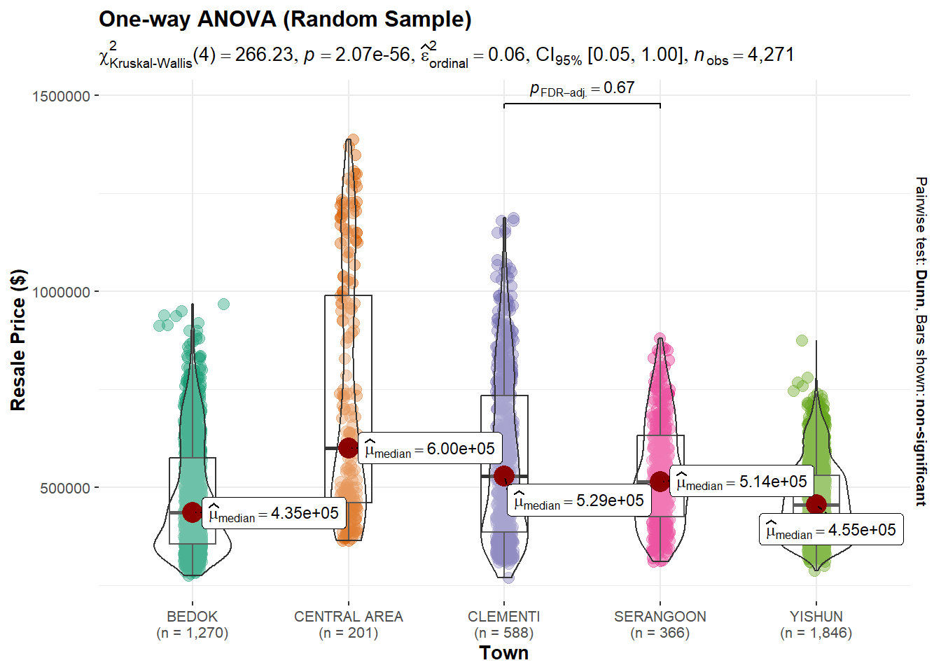
From the test results, we can observe that other than clementi (West) and serangoon (North-East), the median is proven statiscally to be different across towns in the other regions.
4.2.2 HDB flats with larger floor area have higher average resale prices
Intuitively, we expect larger flats will have higher resale price as the purchase price was already higher. However, we can use the data from HDB to test our basis using the transaction data in Year 2022 as shown below.
plot_ly(
  data = HDBdata2022,
  x = ~floor_area_sqm, y = ~resale_price,
  color = ~flat_type,
  type = 'scatter', mode = "markers",
  hovertemplate = ~paste("Floor Area (sqm):", floor_area_sqm,
                         "<br>Resale Price($M):", round(resale_price/1000000,
                                                        digits=2))) |>
#Configure title and axes
  layout(title = "Resale Price vs Floor Area, 2022",
         xaxis = list(title = "Floor Area (sqm)"),
         yaxis = list(title = "Resale Price($)"))
Observations:
The first observation is that the average resale prices increases as the floor area increases.
The second observation is the each flat type can be classified by distinct floor area range.
To test the first observation, the following null hypothesis were tested:
H0: The average resale price for different floor areas are the same.
H1: The average resale price for different floor areas are different.
#check for normality using Anderson-Darling
ad.test(HDBdata2022$floor_area_sqm)
    Anderson-Darling normality test

data:  HDBdata2022$floor_area_sqm
A = 320.42, p-value < 2.2e-16
The Anderson-Darling test output suggest that there is sufficient evidence statistically to reject the null hypothesis that floor area is normally distributed. Therefore, a non-parametric test is used in ggscatterstats() to build a visual for Significant Test of Correlation between Resale Price and Floor Area.
ggscatterstats(
  data = HDBdata2022,
  x = floor_area_sqm,
  y = resale_price,
  type = "nonparametric",
  marginal = TRUE,
  title = "Significant Test of Correlation",
  xlab = "Floor Area (sqm)",
  ylab = "Resale Price ($)"
)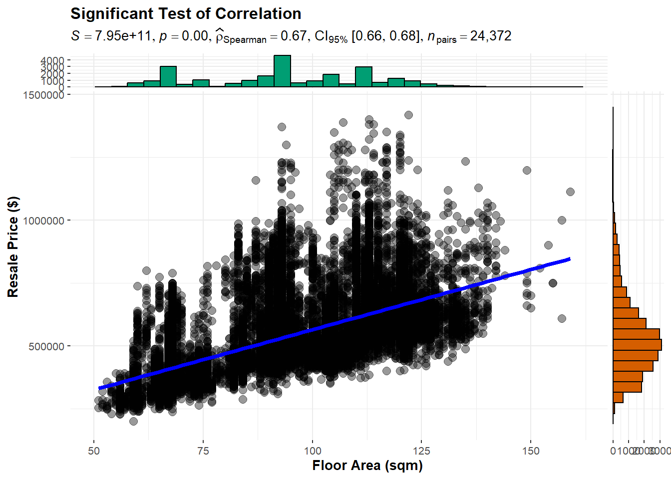
As the test reveals that p-value is less than 𝞪-value, there is sufficient statistical evidence to reject the null hypothesis and conclude that the average resale price between different flat areas are different.
Also, we can conclude intuitively as well as statically that more rooms flat type will fetch higher resale price since each flat type belongs to a relatively distinct floor area range.
4.2.3 HDB flats with higher storey ranges have higher average resale prices
tooltip <- function(y, ymax, accuracy = 1) {   #<<
  mean <- scales::number(y, accuracy = accuracy) #<<
  sem <- scales::number(ymax - y, accuracy = accuracy) #<<
  paste("Average Resale Price($k):", mean, "+/-", sem) #<<
} #<<

gg_point <- ggplot(data=HDBdata2022,
                   aes(x = storey_range),
) +
  stat_summary(aes(y = resale_price/1000,
                   tooltip = after_stat(  #<<
                     tooltip(y, ymax))),  #<<
    fun.data = "mean_se",
    geom = GeomInteractiveCol,  #<<
    fill = "Grey"
  ) +
  stat_summary(aes(y = resale_price/1000),
    fun.data = mean_se,
    geom = "errorbar", width = 0.2, linewidth = 0.2
  ) +
  coord_flip() +
  labs(title="Average Resale Price vs Storey Range, 2022") +
  ylab("Average Resale Price ($k)") +
  xlab("Storey Reange") +
  theme_minimal()

girafe(ggobj = gg_point,
       width_svg = 8,
       height_svg = 8*0.618)
Observations:
It can be observed that the average resale prices for HDB flats increases as the storey ranges increases. This could be due to homeowners wish to stay higher so they are further away from the noise pollution from the roads and human traffic at the ground level.
Another point to note is that the range of the resale price is smaller at the lower storey ranges. This could be due to lower demand, partly caused by the requirements that a minority ethic group can only sell their home to another minority ethic group.
4.2.3 HDB flats models do not show distinct relationship with resale prices
p_boxplot <- HDBdata2022 %>%
  ggplot(aes(x = flat_model, y = resale_price)) +
  geom_boxplot(aes(fill = flat_type)) +
  coord_flip()

ggplotly(p_boxplot) %>%
  layout(title = 'Flat Model vs Resale Price, 2022',
         xaxis = list(title = 'Resale Price'),
         yaxis = list(title = 'Flat Model'),
         legend = list(title=list(text='<b> Flat Type </b>')))
5. Conclusion
From the overall trends, we had observed that overall HDB flat resale prices were on a rise in the year 2022. Towns with newer flats (i.e. longer remaining lease period) generally have higher transaction volume than those with older flats. Diving deeper into factors that could impact resale price, we tested and proven that the median resale prices in the central region are higher than the rest and the mean resale price increases with larger floor area.
If given more time, there are many opportunities to further explore this data set. They include statistically testing on resale price and storey level range and remaining lease as well as visualisation of uncertainty in using price averages in Section 4.1