pacman::p_load(seriation, dendextend, heatmaply, GGally, parallelPlot, tidyverse)In-Class Excerise 5
Installing and Launching R Packages
Importing and Preparing The Data
Importing data set
wh <- read_csv("data/WHData-2018.csv")Preparing the data
row.names(wh) <- wh$CountryTransforming the data frame into matrix
wh1 <- dplyr::select(wh, c(3, 7:12))
wh_matrix <- data.matrix(wh)
Heatmap
Plotting static heatmap
wh_heatmap <- heatmap(wh_matrix,
                      scale="column",
                      cexRow = 0.6,
                      cexCol = 0.8,
                      margins = c(10, 4))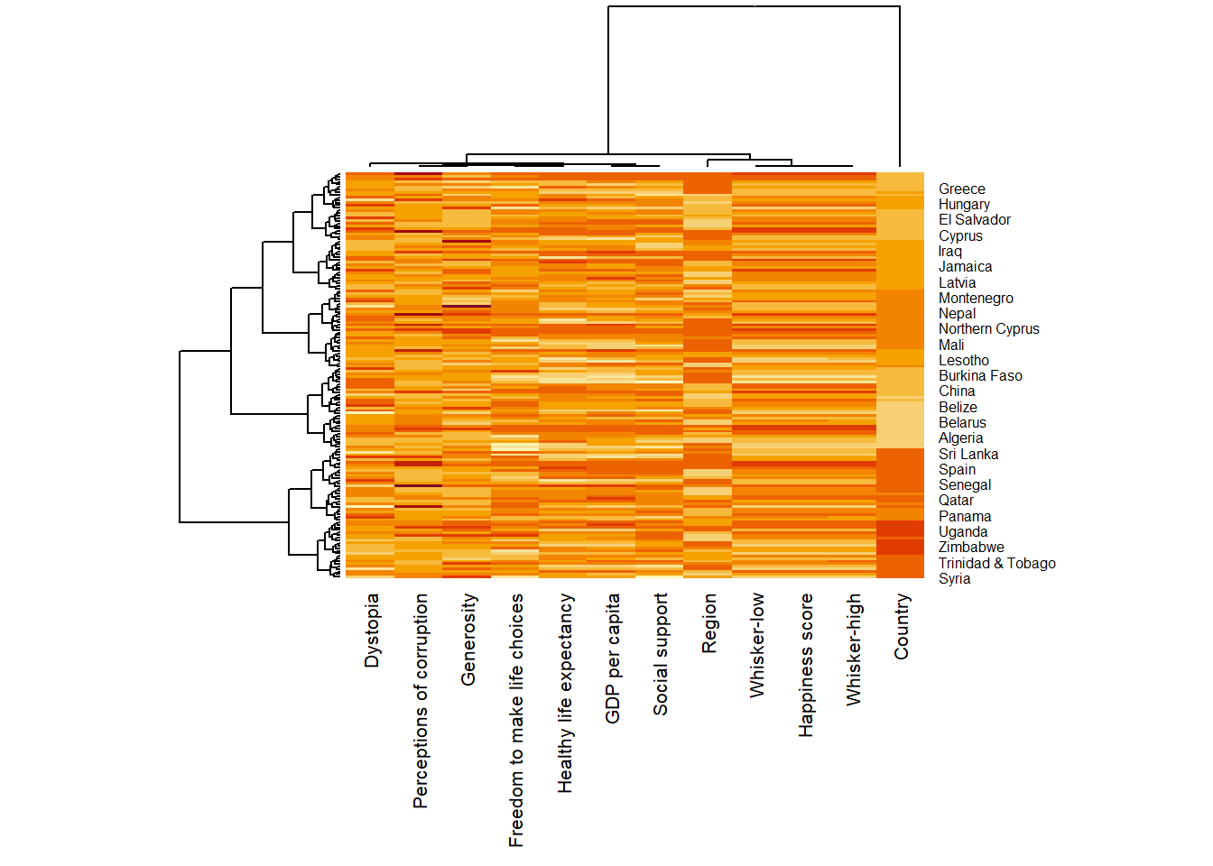
Creating interactive heatmap
heatmaply(wh_matrix[, -c(1, 2, 4, 5)],
          scale = "column")
Clustering
Plotting heatmap by using hierachical clustering algorithm with “Euclidean distance” and “ward.D” method.
heatmaply(normalize(wh_matrix[, -c(1, 2, 4, 5)]),
          dist_method = "euclidean",
          hclust_method = "ward.D")
dend_expend() will be used to determine the recommended clustering method to be used.
wh_d <- dist(normalize(wh_matrix[, -c(1, 2, 4, 5)]), method = "euclidean")
dend_expend(wh_d)[[3]]
dist_methods hclust_methods optim
1 unknown ward.D 0.6137851
2 unknown ward.D2 0.6289186
3 unknown single 0.4774362
4 unknown complete 0.6434009
5 unknown average 0.6701688
6 unknown mcquitty 0.5020102
7 unknown median 0.5901833
8 unknown centroid 0.6338734find_k() is used to determine the optimal number of cluster
wh_clust <- hclust(wh_d, method = "average")
num_k <- find_k(wh_clust)
plot(num_k)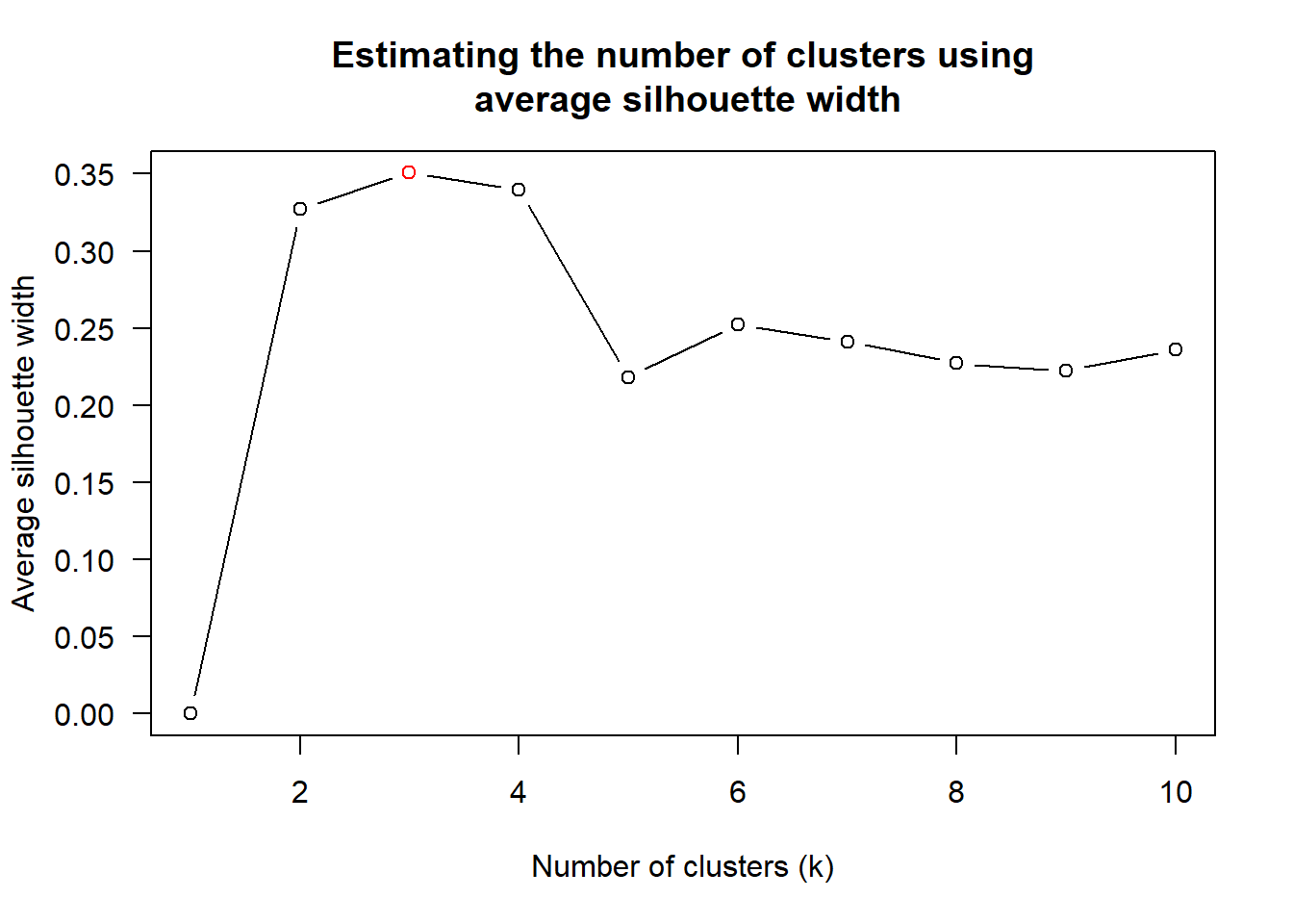
Visualising the clustering
heatmaply(normalize(wh_matrix[, -c(1, 2, 4, 5)]),
          dist_method = "euclidean",
          hclust_method = "average",
          k_row = 3)
Using Blue color paletter of rColorBrewer
heatmaply(normalize(wh_matrix[, -c(1, 2, 4, 5)]),
          seriate = "none",
          colors = Blues)
Adding plotting features to ensure cartographic quality:
k_row is used to produce 5 groups.
margins is used to change the top margin to 60 and row margin to 200.
fontsizw_row and fontsize_col are used to change the font size for row and column labels to 4.
main is used to write the main title of the plot.
xlab and ylab are used to write the x-axis and y-axis labels respectively.
heatmaply(normalize(wh_matrix[, -c(1, 2, 4, 5)]),
          Colv=NA,
          seriate = "none",
          colors = Blues,
          k_row = 5,
          margins = c(NA,200,60,NA),
          fontsize_row = 4,
          fontsize_col = 5,
          main="World Happiness Score and Variables by Country, 2018 \nDataTransformation using Normalise Method",
          xlab = "World Happiness Indicators",
          ylab = "World Countries"
          )
Parallel Coordinates Plot
Plotting basic static parallel coordinates
ggparcoord(data = wh,
           columns = c(7:12))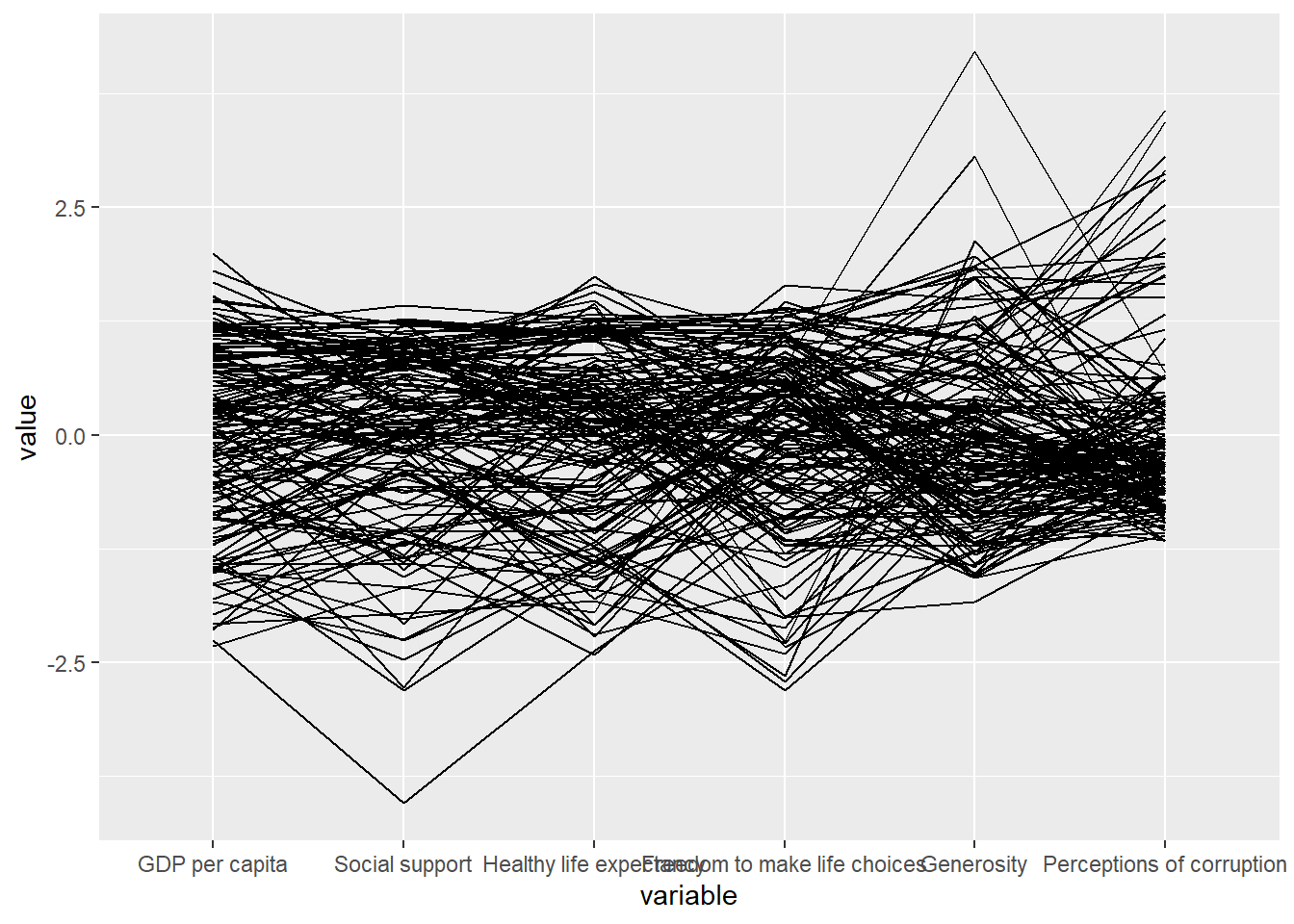
Adding boxplot
ggparcoord(data = wh,
           columns = c(7:12),
           groupColumn = 2,
           scale = "uniminmax",
           alphaLines = 0.2,
           boxplot = TRUE,
           title = "Parallel Coordinates Plot of World Happines Variables")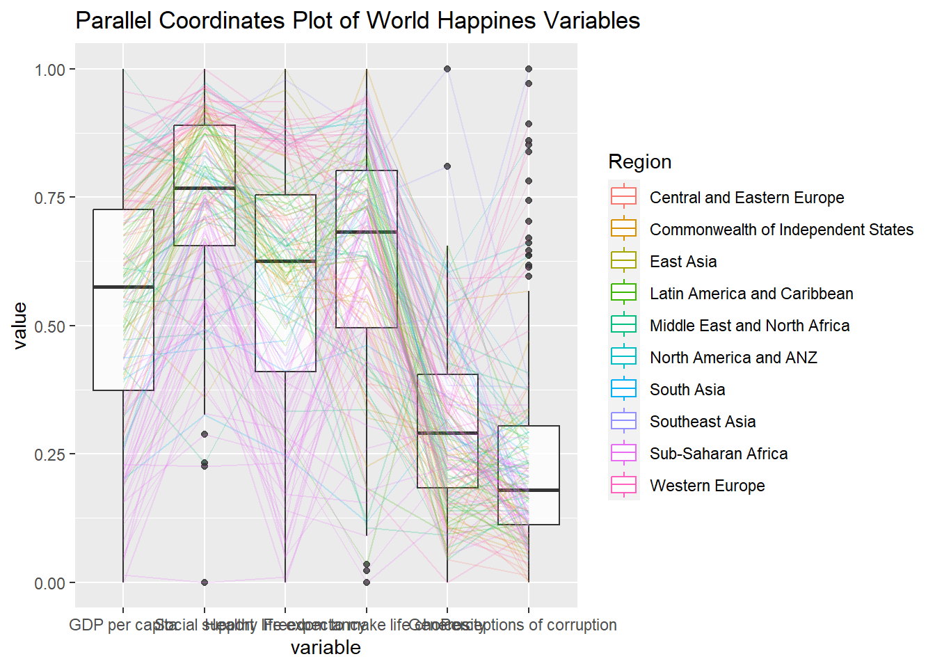
Learning points:
groupColumnargument is used to group the observations (i.e. parallel lines) by using a single variable (i.e. Region) and colour the parallel coordinates lines by region name.scaleargument is used to scale the variables in the parallel coordinate plot by usinguniminmaxmethod. The method univariately scale each variable so the minimum of the variable is zero and the maximum is one.alphaLinesargument is used to reduce the intensity of the line colour to 0.2. The permissible value range is between 0 to 1.boxplotargument is used to turn on the boxplot by using logicalTRUE. The default isFALSE.
Parallel coordinates with facet
ggparcoord(data = wh,
           columns = c(7:12),
           groupColumn = 2,
           scale = "uniminmax",
           alphaLines = 0.2,
           boxplot = TRUE,
           title = "Multiple Parallel Coordinates Plots of World Happines Variables by Region") +
  facet_wrap(~ Region) +
  theme(axis.text.x = element_text(angle = 30, hjust=1))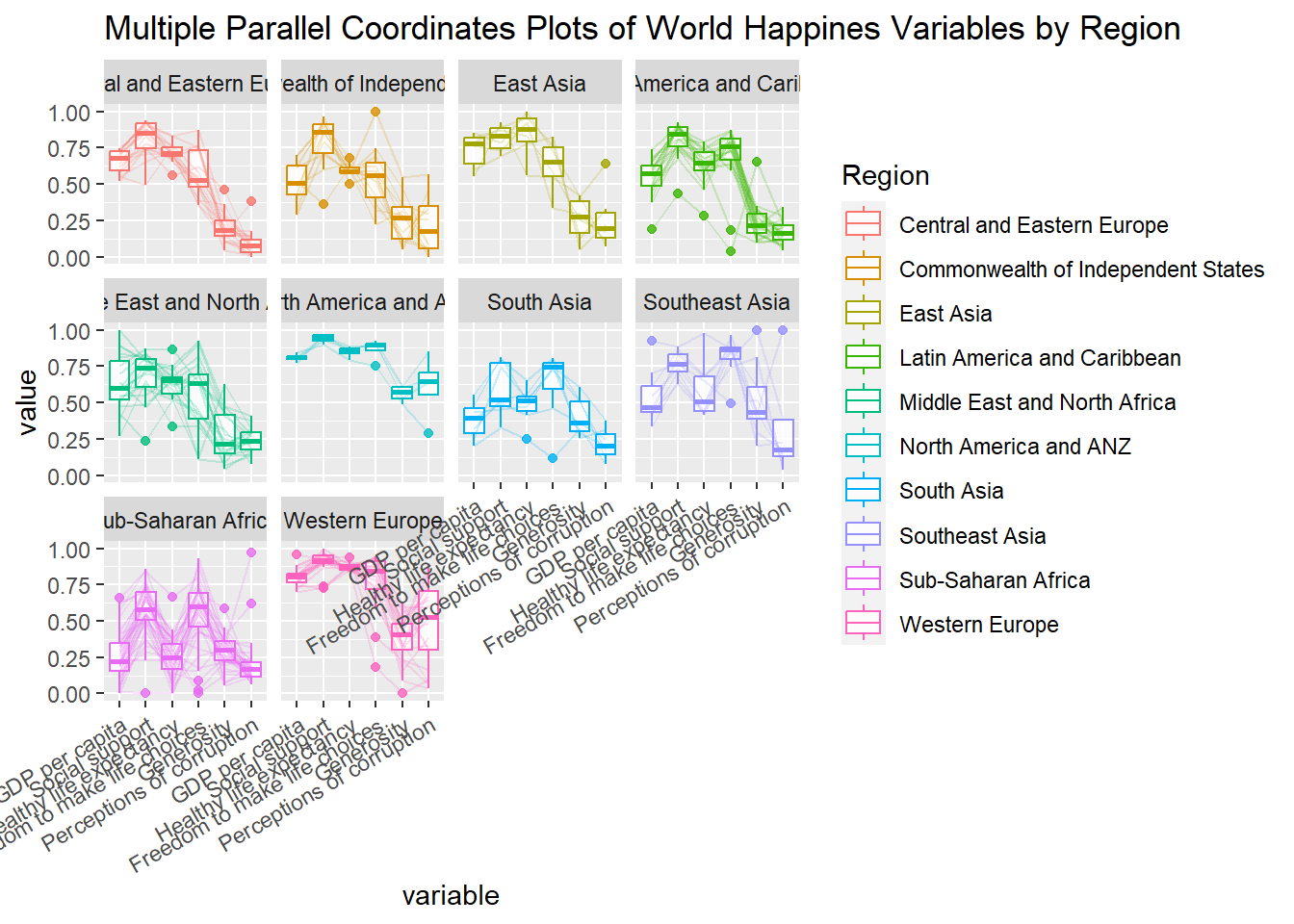
Plotting Interactive Parallel Coordinates Plot
Basic plot
parallelPlot(wh,
             continuousCS = "YlOrRd",
             rotateTitle = TRUE)
Adding histogram
histoVisibility <- rep(TRUE, ncol(wh))
parallelPlot(wh,
             rotateTitle = TRUE,
             histoVisibility = histoVisibility)